PivotTable in Excel: A Practical Step-by-Step Guide
Learn to create, customize, and analyze a pivottable in excel with hands-on steps, examples, and practical tips for cleaner data and faster insights.

A pivot table in Excel lets you summarize large datasets quickly by dragging fields into rows, columns, values, and filters. With this guide, you'll create your first pivottable in excel, refine layouts, and analyze trends without complex formulas. You’ll learn practical steps, common mistakes to avoid, and how to share results with stakeholders.
Why Pivot Tables in Excel Matter
Pivot tables are a foundational tool in Excel for turning large, messy datasets into concise, actionable summaries. A pivottable in excel lets you quickly group data by category, compare metrics, and reveal patterns without writing complex formulas. According to XLS Library, this capability is essential for both aspiring analysts and seasoned professionals who want to explore data interactively. When you start with clean data, a pivottable in excel becomes a flexible canvas where you can experiment with rows, columns, and value calculations to answer business questions in minutes rather than hours.
Key ideas:
- Speed: summarize thousands of rows with a few clicks
- Flexibility: reconfigure your view on the fly
- Clarity: reduce noise and highlight meaningful trends
In practice, pivottable in excel work best when you maintain consistent headers and avoid merged cells, so Excel can automatically detect field names and aggregate correctly.
Understanding the Pivot Table Anatomy
A pivot table in Excel comprises four core areas: Rows, Columns, Values, and Filters. Dragging a field into Rows defines how data is grouped; placing a field in Columns creates column-wise summaries; Values are the numeric calculations that power your insights; Filters let you narrow the data set without changing the pivot structure. In a pivottable in excel, you can switch betweenSum, Count, Average, and more, depending on what you want to measure. This modular design makes it easy to compare regions, products, time periods, or customer segments side by side. As you rearrange fields, you’ll immediately see the impact on totals, subtotals, and grand totals, enabling rapid hypothesis testing.
Preparing Your Data for Pivot Tables
Your pivot table relies on clean, well-structured data. Before you create a pivottable in excel, ensure headers are unique, data types are consistent, and there are no blank rows in the main data area. Convert the data range into a formal Excel Table (Ctrl+T) to gain automatic expansion as you add new records. Based on XLS Library Analysis, 2026, well-prepared data reduces refresh errors and improves performance when you build a pivottable in excel. Keep a separate sheet with a data dictionary if your workbook will be shared, so teammates know what each column represents.
Checklist:
- One header row, no merged cells
- Consistent numbers, dates, and text
- No stray spaces or non-printing characters in headers
With these basics, your pivottable in excel will be ready for clean, reliable analysis.
Step-by-Step Overview for Quick Results
To get started with a pivottable in excel, you’ll typically follow a small, logical loop: identify your question, assemble the data, and then validate the output. This section provides a high-level overview so you can understand the flow before diving into the full steps. Expect to introduce rows and columns, add a value measure, and apply a filter or slicer to focus the view. The beauty of a pivottable in excel is that you can reshape the same dataset to reveal different angles without touching the raw data. The steps below expand this overview into concrete actions when you’re ready to implement in your workbook.
Practical Example: Sales Data Analysis
Imagine a sales dataset with fields like Region, Product, Date, and SalesAmount. A pivottable in excel can instantly show total sales by Region, then break it down by Product, or by Month for time-based trends. By dragging Region into Rows, Product into Columns, and SalesAmount into Values (summed), you’ll see a compact matrix of totals. Add Date as a Filter to compare current-quarter performance with prior periods. This practical example demonstrates how a pivottable in excel accelerates decision-making by turning raw records into readable dashboards.
Common Pitfalls and How to Avoid Them
Even skilled analysts stumble with pivot tables if the data foundation isn’t solid. Common pitfalls include relying on merged cells, ignoring data types, and using inconsistent headers. For a pivottable in excel, ensure your source data stays in a tabular format, headers are exact text, and there are no blank columns or rows inside the data range. Another pitfall is overloading the pivot with too many fields, which can blur insights; keep the view focused and group related fields. Finally, remember to refresh the pivot when the source data changes, otherwise your results will be out of date.
Advanced Techniques: Calculated Fields, Slicers, and More
As you gain familiarity with the pivottable in excel, you can push its power with calculated fields, which let you define new metrics with simple formulas inside the pivot. Slicers and timeline controls add interactivity to dashboards, allowing stakeholders to filter by category, region, or date range with a click. If you’re comfortable with data modeling, enable the Data Model (Power Pivot) to relate multiple tables without duplicating data. These techniques expand the pivottable in excel beyond basic summarization into a full data-analysis toolkit.
Pivot Tables Across Excel Versions and Data Sources
Microsoft Excel’s pivot functionality remains consistent across recent versions, including Excel for Microsoft 365, Excel 2019, and Excel Online. The core concepts of Rows, Columns, Values, and Filters stay the same, but performance and feature availability vary. For multi-table analyses, use the Data Model to create relationships between tables and build richer pivot reports using the pivottable in excel as your central analysis layer. When working with external data sources, you can import data via Power Query and refresh your pivottable in excel with the latest results.
If you rely on older workbooks, consider upgrading or using compatibility settings to preserve functionality while you learn advanced pivottable in excel capabilities.
Integrating Pivot Tables with Charts and Dashboards
Pivot tables are often the backbone of dashboards because they feed cleanly into charts and slicers. Create a pivot chart from your pivottable in excel to visualize trends and performance side by side with summary tables. Use conditional formatting to highlight key values and create a compelling narrative for stakeholders. As you publish dashboards, ensure your viewers understand the data source and refresh cadence. The pivottable in excel, when paired with visuals, becomes a powerful storytelling tool for business insights.
Tools & Materials
- Computer with Windows or macOS(Any modern machine will do)
- Microsoft Excel (365 or 2019+)(PivotTable support required)
- Raw data in a clean Excel table or CSV(Headers in first row; no merged cells)
- Stable data source sheet(Keep data in a single range or table)
- Backup copy of data(Before you start pivoting)
- Optional: Data Model / Power Pivot add-in(For multi-table relationships)
- Data dictionary or column descriptions(Helpful for collaborators)
Steps
Estimated time: Total time: 20-30 minutes
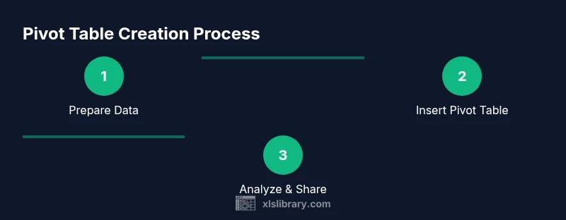
- 1
Prepare the data
Ensure your data is in a clean, tabular format with a single header row. Remove merged cells, convert the range to a formal Excel Table (Ctrl+T), and verify data types are consistent across each column. These steps prevent common refresh errors when building a pivottable in excel.
Tip: Convert to a table to automatically expand with new data. - 2
Insert the Pivot Table
Select a cell in the data and go to Insert > PivotTable. Choose whether to place the pivot on a new worksheet or the existing sheet. This creates the pivottable in excel shell ready for field placement.
Tip: Choose New Worksheet for clarity and future editing. - 3
Add Fields to Rows and Columns
Drag the desired fields into the Rows and Columns areas to define your layout. Use a few high-cardinality fields in Rows and aggregate fields in Values to keep the pivot readable. This setup drives clear comparisons in pivottable in excel.
Tip: Right-click a field to adjust sorting and grouping. - 4
Add Values and summarize
Place numeric fields into Values and choose Sum, Count, or Average as appropriate. Formatting options let you show currency, thousands separators, and decimals. This step defines the core metric you’ll analyze in pivottable in excel.
Tip: Use Value Field Settings to tailor aggregation. - 5
Apply Filters and Slicers
Add filters to confine the data by category or date. Slicers offer a modern, interactive way to filter dashboards, which is especially helpful for stakeholders. Keep the filter set tight to preserve readability in pivottable in excel.
Tip: Keep slicers focused to avoid clutter. - 6
Format and customize
Adjust number formats, font styles, and layout options to improve readability. Subtotals and grand totals can be hidden or shown based on your needs. Tidy presentation helps stakeholders understand pivottable in excel results at a glance.
Tip: Use Report Layout: Show in Tabular Form for clarity. - 7
Analyze, save, and share
Review results, validate against source data, and save the workbook. If needed, export insights to PDF or share the live workbook with colleagues. Always note the data source and refresh cadence when sharing pivottable in excel results.
Tip: Always refresh before presenting results.
People Also Ask
What is a PivotTable and why would I use it?
A PivotTable is a dynamic summary tool that lets you reorganize and summarize selected columns and rows of data to obtain a desired report. It makes it easy to facet data by categories and measure performance across multiple dimensions without changing the underlying dataset.
A PivotTable is a dynamic summary tool that helps you reorganize data to see trends and differences across categories, without altering the original data.
What data quality steps are essential before creating a PivotTable?
Ensure headers are unique, data types are consistent, and there are no blank rows in the main data area. Avoid merged cells in the source data and convert the range to a table for reliability.
Make sure headers are clear and data types are consistent before building a PivotTable to avoid errors.
Can PivotTables pull from multiple data sources?
PivotTables can work with a single source effectively. For multiple sources, use the Data Model (Power Pivot) to relate tables and create richer pivots.
If you have multiple data sources, enable the Data Model to relate them and build multi-table pivots.
How do I refresh a PivotTable after data updates?
Click Refresh on the PivotTable Tools ribbon or press Alt+F5 to update results. Verify the data source range includes all new records.
Refresh the PivotTable to reflect changes by using the Refresh option on the ribbon.
What are calculated fields and when should I use them?
Calculated fields let you create custom metrics inside the PivotTable with simple formulas. Use them when you need on-the-fly calculations without altering source data.
Calculated fields add new metrics directly inside the PivotTable for quick, on-demand analysis.
How can I share PivotTable results with others?
Export the workbook or create a static report, then share a link or PDF. For interactive sharing, consider providing a dashboard-enabled workbook.
Share the workbook or export your pivot-based report for others to view.
Watch Video
The Essentials
- Start with clean, tabular data to fuel reliable pivots.
- Place essential fields in Rows/Columns and summarize with Values.
- Use Filters or Slicers to refine insights without changing data.
- Leverage the Data Model for multi-table pivots and advanced analysis.
- Pair pivots with charts to build effective dashboards.